DFE inference
import pickle, random
import numpy as np
import nlopt
import dadi
import dadi.DFE as DFE
import matplotlib.pyplot as plt
from dadi.DFE import *
1D examples
# For multiprocessing to work on Windows, all script code must be wrapped
# in this block. If you're not on Windows, feel free to remove this if statement.
if __name__ == '__main__':
    # Set demographic parameters and theta. This is usually inferred from
    # synonymous sites. In this case, we'll be using a two-epoch model.
    demog_params = [2, 0.05]
    theta_ns = 4000.
    ns = [250]

    # Integrate over a range of gammas
    #pts_l = [600, 800, 1000]
    #spectra = DFE.Cache1D(demog_params, ns, DFE.DemogSelModels.two_epoch, pts_l=pts_l,
    #                      gamma_bounds=(1e-5, 500), gamma_pts=100, verbose=True,
    #                      mp=True)
    # The spectra can be pickled for usage later. This is especially convenient
    # if the process of generating the spectra takes a long time.
    #pickle.dump(spectra, open('example_spectra.bpkl','wb'))
    # To load them, use this code
    spectra = pickle.load(open('example_spectra.bpkl','rb'))
#load sample data
data = dadi.Spectrum.from_file('example.fs')

# Fit a DFE to the data
# Initial guess and bounds
sel_params = [0.2, 1000.]
lower_bound, upper_bound = [1e-3, 1e-2], [1, 50000.]
p0 = dadi.Misc.perturb_params(sel_params, lower_bound=lower_bound,
                              upper_bound=upper_bound)
popt = dadi.Inference.opt(p0, data, spectra.integrate, pts=None,
                          func_args=[DFE.PDFs.gamma, theta_ns],
                          lower_bound=lower_bound, upper_bound=upper_bound,
                          verbose=len(sel_params), maxiter=10, multinom=False)

# Get expected SFS for MLE
model_sfs = spectra.integrate(popt, None, DFE.PDFs.gamma, theta_ns, None)
# One possible characterization of the neutral+gamma DFE
# Written using numpy tricks to work with both scalar and array arguments
def neugamma(xx, params):
    pneu, alpha, beta = params
    # Convert xx to an array
    xx = np.atleast_1d(xx)
    out = (1-pneu)*DFE.PDFs.gamma(xx, (alpha, beta))
    # Assume gamma < 1e-4 is essentially neutral
    out[np.logical_and(0 <= xx, xx < 1e-4)] += pneu/1e-4
    # Reduce xx back to scalar if it's possible
    return np.squeeze(out)

sel_params = [0.2, 0.2, 1000.]
lower_bound, upper_bound = [1e-3, 1e-3, 1e-2], [1, 1, 50000.]
p0 = dadi.Misc.perturb_params(sel_params, lower_bound=lower_bound,
                              upper_bound=upper_bound)
popt = dadi.Inference.opt(p0, data, spectra.integrate, pts=None,
                          func_args=[neugamma, theta_ns],
                          lower_bound=lower_bound, upper_bound=upper_bound,
                          verbose=len(sel_params),
                          maxiter=10, multinom=False)
#
# Modeling ancestral state misidentification, using dadi's built-in function to
# wrap fitdadi's integrate method.
#
p_misid = 0.05
data = dadi.Numerics.apply_anc_state_misid(data, p_misid)
misid_func = dadi.Numerics.make_anc_state_misid_func(spectra.integrate)
sel_params = [0.2, 1000., 0.2]
lower_bound, upper_bound = [1e-3, 1e-2, 0], [1, 50000., 1]
p0 = dadi.Misc.perturb_params(sel_params, lower_bound=lower_bound,
                              upper_bound=upper_bound)
popt = dadi.Inference.opt(p0, data, misid_func, pts=None,
                          func_args=[DFE.PDFs.gamma, theta_ns],
                          lower_bound=lower_bound, upper_bound=upper_bound,
                          verbose=len(sel_params), maxiter=10,
                          multinom=False)
#
# Including a point mass of positive selection
#
data = dadi.Spectrum.from_file('example.fs')
ppos = 0.1
sel_data = theta_ns*DFE.DemogSelModels.two_epoch(tuple(demog_params) + (5,), ns, pts_l[-1])
data_pos = (1-ppos)*data + ppos*sel_data

sel_params = [0.2, 1000., 0.2, 2]
lower_bound, upper_bound = [1e-3, 1e-2, 0, 0], [1, 50000., 1, 50]
p0 = dadi.Misc.perturb_params(sel_params, lower_bound=lower_bound,
                              upper_bound=upper_bound)
popt = dadi.Inference.opt(p0, data_pos, spectra.integrate_point_pos, pts=None,
                          func_args=[DFE.PDFs.gamma, theta_ns, DFE.DemogSelModels.two_epoch],
                          lower_bound=lower_bound, upper_bound=upper_bound,
                          verbose=len(sel_params), maxiter=10, multinom=False)
#
# Multiple point masses of positive selection
#
# Parameters are mu, sigma, ppops1, gammapos1, ppos2, gammapos2
sel_params = [3,2,0.1,2,0.3,6]
input_fs = spectra.integrate_point_pos(sel_params,None,DFE.PDFs.lognormal,theta_ns,
                                       DFE.DemogSelModels.two_epoch, 2)
data = input_fs.sample()
lower_bound, upper_bound = [-1,0.1,0,0,0,0], [5,5,1,10,1,20]
p0 = dadi.Misc.perturb_params(sel_params, lower_bound=lower_bound,
                              upper_bound=upper_bound)

def ieq_constraint(p,*args):
    # Our constraint is that ppop1+ppos2 must be less than 1.
    return [1-(p[2]-p[4])]

popt = dadi.Inference.opt(p0, data, spectra.integrate_point_pos, pts=None,
                          func_args=[DFE.PDFs.lognormal, theta_ns,
                                     DFE.DemogSelModels.two_epoch, 2],
                          lower_bound=lower_bound, upper_bound=upper_bound,
                          ieq_constraint=ieq_constraint,
                          # Fix gammapos1
                          fixed_params=[None,None,None,2,None,None],
                          verbose=len(sel_params),
                          maxiter=10, multinom=False)
2D examples
# Seed random number generator, so example is reproducible
np.random.seed(1398238)
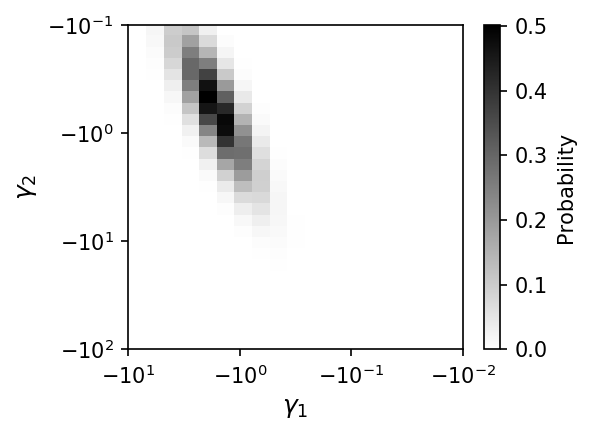
#
# Plotting a joint DFE
#
sel_dist = PDFs.biv_lognormal
params = [0.5,-0.5,0.5,1,-0.8]
gammax, gammay = -np.logspace(-2, 1, 20), -np.logspace(-1, 2, 30)
fig = plt.figure(137, figsize=(4,3), dpi=150)
fig.clear()
ax = fig.add_subplot(1,1,1)
Plotting.plot_biv_dfe(gammax, gammay, sel_dist, params, logweight=True, ax=ax)
fig.tight_layout()
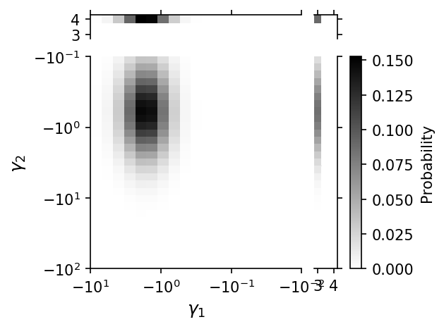
# With positive selection
params = [0.5,-0.5,0.5,1,0.0,0.3,3,0.3,4]
fig = Plotting.plot_biv_point_pos_dfe(gammax, gammay, sel_dist, params,
                                      fignum=23, rho=params[4])
# For multiprocessing to work on Windows, all script code must be wrapped
# in this block. If you're not on Windows, feel free to remove this if statement.
if __name__ == '__main__':
    #
    # Full test of optimization machinery.
    # Considering only a narrow range of gammas, so integration is faster.
    #
    demo_params = [0.5,2,0.5,0.1,0,0]
    ns = [8, 12]
    pts_l = [60, 80, 100]
    func_ex = DemogSelModels.IM
    # Check whether we already have a chached set of 2d spectra. If not
    # generate them.
    try:
        s2 = pickle.load(open('test.spectra2d.bpkl', 'rb'))
    except IOError:
        s2 = Cache2D(demo_params, ns, func_ex, pts=pts_l, gamma_pts=100,
                     gamma_bounds=(1e-2, 10), verbose=True, mp=True,
                     additional_gammas=[1.2, 4.3])
        # Save spectra2d object
        fid = open('test.spectra2d.bpkl', 'wb')
        pickle.dump(s2, fid, protocol=2)
        fid.close()

        ## Cache generation can be very computationally expensive, even
        ## with multiprocessing. If you need to split the work across multiple
        ## compute nodes, use the split_jobs and this_job_id arguments, then
        ## merge the partial caches.
        ## In this example, the 3 partial caches could be generate on independent
        ## nodes, then s2a,s2b,s2c would be saved to separate files, then loaded
        ## and combined later.
        #s2a = Cache2D(demo_params, ns, func_ex, pts=pts_l, gamma_pts=100,
        #        gamma_bounds=(1e-2, 10), verbose=True, mp=True,
        #        additional_gammas=[1.2, 4.3], split_jobs=3, this_job_id=0)
        #s2b = Cache2D(demo_params, ns, func_ex, pts=pts_l, gamma_pts=100,
        #        gamma_bounds=(1e-2, 10), verbose=True, mp=True,
        #        additional_gammas=[1.2, 4.3], split_jobs=3, this_job_id=1)
        #s2c = Cache2D(demo_params, ns, func_ex, pts=pts_l, gamma_pts=100,
        #        gamma_bounds=(1e-2, 10), verbose=True, mp=True,
        #        additional_gammas=[1.2, 4.3], split_jobs=3, this_job_id=2)
        #s2 = Cache2D.merge([s2a, s2b, s2c])
# Generate test data set to fit
input_params, theta = [0.5,0.5,-0.8], 1e5
sel_dist = PDFs.biv_lognormal
# Expected sfs
target = s2.integrate(input_params, None, sel_dist, theta, None)
# Get data with Poisson variance around expectation
data = target.sample()

# Parameters are mean, variance, and correlation coefficient
p0 = [0,1.,0.8]
popt = dadi.Inference.opt(p0, data, s2.integrate, pts=None,
                          func_args=[sel_dist, theta],
                          lower_bound=[None,0,-1],
                          upper_bound=[None,None,1],
                          verbose=30, multinom=False)
print('Input parameters: {0}'.format(input_params))
print('Optimized parameters: {0}'.format(popt))
480     , -2651.22    , array([ 0.712271   ,  0.304346   ,  0.592511   ])
510     , -740.865    , array([ 0.541592   ,  0.790878   ,  0.520651   ])
540     , -519.63     , array([ 0.497606   ,  0.512338   , -0.64606    ])
570     , -519.624    , array([ 0.497503   ,  0.510381   , -0.665866   ])
600     , -519.624    , array([ 0.497503   ,  0.510381   , -0.665865   ])
630     , -519.624    , array([ 0.497503   ,  0.510381   , -0.665865   ])
660     , -519.624    , array([ 0.497503   ,  0.510381   , -0.665865   ])
690     , -519.624    , array([ 0.497503   ,  0.510381   , -0.665865   ])
720     , -519.624    , array([ 0.497503   ,  0.510381   , -0.665865   ])
Input parameters: [0.5, 0.5, -0.8]
Optimized parameters: [ 0.49750313  0.51038084 -0.66686542]
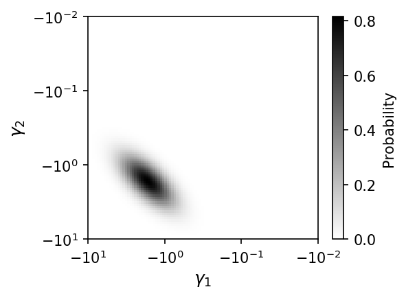
# Plot inferred DFE. Note that this will render slowly, because grid of
# gammas is fairly dense.
fig = plt.figure(231, figsize=(4,3), dpi=150)
fig.clear()
ax = fig.add_subplot(1,1,1)
Plotting.plot_biv_dfe(s2.gammas, s2.gammas, sel_dist, popt, ax=ax)
fig.tight_layout()
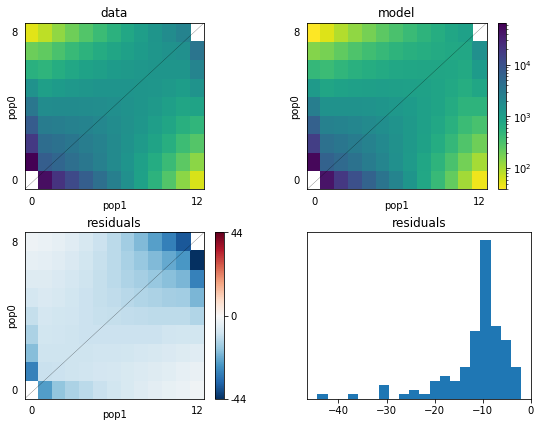
#
# Test point mass of positive selection. To do so, we test against
# the single-population case using very high correlation.
#
params = [-0.5,0.5,0.99, 0.1, 4.3]
fs_biv = s2.integrate_symmetric_point_pos(params, None, PDFs.biv_lognormal, theta,
                                          pts=None)

func_single_ex = DemogSelModels.IM_single_gamma
try:
    s1 = pickle.load(open('test.spectra1d.bpkl', 'rb'))
except IOError:
    s1 = Cache1D(demo_params, ns, func_single_ex, pts_l=pts_l,
                 gamma_pts=100, gamma_bounds=(1e-2, 10), mp=True,
                 additional_gammas = [1.2, 4.3], verbose=False)
    fid = open('test.spectra1d.bpkl', 'wb')
    pickle.dump(s1, fid, protocol=2)
    fid.close()

fs1 = s1.integrate_point_pos([-0.5,0.5,0.1,4.3], None, PDFs.lognormal,
                             1e5, func_single_ex)

fig = dadi.Plotting.pylab.figure(figsize=(8,6))
fig.clear()
dadi.Plotting.plot_2d_comp_Poisson(fs1, fs_biv, show=False)
#
# Test optimization of point mass positive selection.
#

# Generate test data set to fit
# This is a symmetric case, with mu1=mu2=0.5, sigma1=sigma2=0.3, rho=-0.5,
# ppos1=ppos2=0.2, gammapos1=gammapos2=1.2.
input_params, theta = [0.5,0.3,-0.5,0.2,1.2], 1e5
# Expected sfs
target = s2.integrate_symmetric_point_pos(input_params, None, sel_dist, theta,
                                          pts=None)
# Get data with Poisson variance around expectation
data = target.sample()

# We'll fit using our special-case symmetric function. The last
# two arguments are ppos and gammapos. The first three are thus for the
# lognormal distribution. Note that our lognormal distribution assumes
# symmetry if the length of the arguments is only three. If we wanted
# asymmetric lognormal, we would pass in a p0 of total length 7.
p0 = [0.3,0.3,0.1,0.2,1.2]
popt = dadi.Inference.opt(p0, data,
                          s2.integrate_symmetric_point_pos,
                          pts=None, func_args=[sel_dist, theta],
                          # Note that mu in principle has no lower or
                          # upper bound, sigma has only a lower bound
                          # of 0, ppos is bounded between 0 and 1, and
                          # gamma pos is bounded from below by 0.
                          lower_bound=[-1,0.1,-1,0,0],
                          upper_bound=[1,1,1,1,None],
                          # We fix the gammapos to be 1.2, because
                          # we can't do this integration effectively
                          # if gammapos is allowed to vary.
                          fixed_params=[None,None,None,None,1.2],
                          verbose=30, multinom=False)
print('Symmetric test fit')
print('  Input parameters: {0}'.format(input_params))
print('  Optimized parameters: {0}'.format(popt))
780     , -728.975    , array([ 0.317945   ,  0.301612   ,  0.0992905  ,  0.139505   ,  1.2        ])
810     , -575.018    , array([ 0.438034   ,  0.538922   , -0.403391   ,  0.173301   ,  1.2        ])
840     , -575.018    , array([ 0.438034   ,  0.538921   , -0.403391   ,  0.173301   ,  1.2        ])
870     , -553.801    , array([ 0.448013   ,  0.430578   , -0.467847   ,  0.18045    ,  1.2        ])
900     , -551.71     , array([ 0.42946    ,  0.434882   , -0.459367   ,  0.178665   ,  1.2        ])
930     , -551.71     , array([ 0.42946    ,  0.434881   , -0.459368   ,  0.178665   ,  1.2        ])
960     , -551.71     , array([ 0.42946    ,  0.434881   , -0.459368   ,  0.178665   ,  1.2        ])
990     , -551.71     , array([ 0.42946    ,  0.434881   , -0.459368   ,  0.178665   ,  1.2        ])
1020    , -551.71     , array([ 0.42946    ,  0.434881   , -0.459368   ,  0.178665   ,  1.2        ])
1050    , -551.71     , array([ 0.42946    ,  0.434881   , -0.459368   ,  0.178665   ,  1.2        ])
1080    , -551.71     , array([ 0.42946    ,  0.434881   , -0.459368   ,  0.178665   ,  1.2        ])
1110    , -551.71     , array([ 0.42946    ,  0.434881   , -0.459368   ,  0.178665   ,  1.2        ])
1140    , -551.71     , array([ 0.42946    ,  0.434881   , -0.459368   ,  0.178665   ,  1.2        ])
1170    , -551.71     , array([ 0.42946    ,  0.434881   , -0.459368   ,  0.178665   ,  1.2        ])
1200    , -551.71     , array([ 0.42946    ,  0.434881   , -0.459368   ,  0.178665   ,  1.2        ])
1230    , -551.71     , array([ 0.42946    ,  0.434881   , -0.459368   ,  0.178665   ,  1.2        ])
1260    , -551.71     , array([ 0.42946    ,  0.434881   , -0.459368   ,  0.178665   ,  1.2        ])
1290    , -551.73     , array([ 0.429022   ,  0.43591    , -0.458862   ,  0.178569   ,  1.2        ])
Symmetric test fit
  Input parameters: [0.5, 0.3, -0.5, 0.2, 1.2]
  Optimized parameters: [ 0.42946048  0.43488087 -0.45936782  0.17866528  1.2       ]
#
# Mixture model
#

# Now a mixture model, which adds together a 2D distribution and a
# perfectly correlated 1D distribution.
# Input parameters here a mu, sigma, rho for 2D (fixed to zero),
#   proportion positive, gamma positive, proportion 2D,
input_params, theta = [0.5,0.3,0,0.2,1.2,0.2], 1e5
# Expected sfs
target = mixture_symmetric_point_pos(input_params,None,s1,s2,PDFs.lognormal,
                                     PDFs.biv_lognormal, theta)
p0 = [0.3,0.3,0,0.2,1.2,0.3]
popt = dadi.Inference.opt(p0, data, mixture_symmetric_point_pos, pts=None,
                          func_args=[s1, s2, PDFs.lognormal,
                                     PDFs.biv_lognormal, theta],
                          lower_bound=[None, 0.1,-1,0,None, 0],
                          upper_bound=[None,None, 1,1,None, 1],
                          # We fix both the rho assumed for the 2D distribution,
                          # and the assumed value of positive selection.
                          fixed_params=[None,None,0,None,1.2,None],
                          verbose=30, multinom=False, maxiter=1)
1320 , -2719 , array([ 0.189489 , 0.293573 , 0 , 0.133956 , 1.2 , 0.439247 ])
#
# Test Godambe code for estimating uncertainties
#
input_params = [0.3,0.3,0.1,0.2,1.2]
# Generate data in segments for future bootstrapping
fs0 = s2.integrate_symmetric_point_pos(input_params, None, sel_dist,
                                       theta/100., pts=None)
# The multiplication of fs0 is to create a range of data size among
# bootstrap chunks, which creates a range of thetas in the bootstrap
# data sets.
data_pieces = [(fs0*(0.5 + (1.5-0.5)/99*ii)).sample() for ii in range(100)]
# Add up those segments to get our data spectrum
data = dadi.Spectrum(np.sum(data_pieces, axis=0))
# Do the optimization
popt = dadi.Inference.opt([0.2,0.2,0.15,0.3,1.2], data,
                          s2.integrate_symmetric_point_pos,
                          pts=None, func_args=[sel_dist, theta],
                          lower_bound=[-1,0.1,-1,0,0],
                          upper_bound=[1,1,1,1,None],
                          fixed_params=[None,None,None,None,1.2],
                          verbose=30, multinom=False)

print('Symmetric test fit')
print('  Input parameters: {0}'.format(input_params))
print('  Optimized parameters: {0}'.format(popt))
1380    , -834.159    , array([ 0.164119   ,  0.462983   , -0.0814004  ,  0.129806   ,  1.2        ])
1410    , -547.791    , array([ 0.211566   ,  0.491704   ,  0.0874909  ,  0.180269   ,  1.2        ])
1440    , -547.791    , array([ 0.211546   ,  0.491728   ,  0.0874776  ,  0.180265   ,  1.2        ])
1470    , -547.791    , array([ 0.211566   ,  0.491704   ,  0.0874909  ,  0.180269   ,  1.2        ])
1500    , -547.791    , array([ 0.211566   ,  0.491704   ,  0.0874909  ,  0.180269   ,  1.2        ])
1530    , -547.791    , array([ 0.211566   ,  0.491704   ,  0.0874909  ,  0.180269   ,  1.2        ])
1560    , -547.791    , array([ 0.211566   ,  0.491704   ,  0.0874909  ,  0.180269   ,  1.2        ])
1590    , -547.791    , array([ 0.211566   ,  0.491704   ,  0.0874909  ,  0.180269   ,  1.2        ])
1620    , -547.791    , array([ 0.211566   ,  0.491704   ,  0.0874909  ,  0.180269   ,  1.2        ])
1650    , -547.791    , array([ 0.211566   ,  0.491704   ,  0.0874909  ,  0.180269   ,  1.2        ])
1680    , -547.791    , array([ 0.211566   ,  0.491704   ,  0.0874909  ,  0.180269   ,  1.2        ])
1710    , -547.791    , array([ 0.211566   ,  0.491704   ,  0.0874909  ,  0.180269   ,  1.2        ])
1740    , -547.791    , array([ 0.211566   ,  0.491704   ,  0.0874909  ,  0.180269   ,  1.2        ])
1770    , -547.791    , array([ 0.211566   ,  0.491704   ,  0.0874909  ,  0.180269   ,  1.2        ])
Symmetric test fit
  Input parameters: [0.3, 0.3, 0.1, 0.2, 1.2]
  Optimized parameters: [0.21156582 0.49170413 0.0874909  0.18026894 1.2       ]
# Generate bootstraps for Godambe
all_boot = []
for boot_ii in range(100):
    # Each bootstrap is made by sampling, with replacement, from our data
    # pieces
    this_pieces = [random.choice(data_pieces) for _ in range(100)]
    all_boot.append(dadi.Spectrum(np.sum(this_pieces, axis=0)))

# The Godambe methods only accept a basic dadi function that takes in
# parameters, ns, and pts. Moreover, we can't allow gammapos to vary.
# (We don't have variations around those cached. We could work around this
# by pre-caching the necessary values, but it would be inelegant.) So
# we create this simple function that holds gammapos constant and removes
# it from the argument list.
def temp_func(pin, ns, pts):
    # Add in gammapos parameter
    params = np.concatenate([pin, [1.2]])
    return s2.integrate_symmetric_point_pos(params, None, sel_dist,
                                            theta, pts=None)

# Run the uncertainty analysis. Note that each bootstrap data set
# needs a different assumed theta. We estimate theta for each bootstrap
# data set simply by scaling theta from the orignal data.
import dadi.Godambe
boot_theta_adjusts = [b.sum()/data.sum() for b in all_boot]
uncerts_adj = dadi.Godambe.GIM_uncert(temp_func, [], all_boot, popt[:-1],
                                      data, multinom=False,
                                      boot_theta_adjusts=boot_theta_adjusts)
print('Godambe uncertainty test')
print('  Input parameters: {0}'.format(input_params))
print('  Optimized parameters: {0}'.format(popt))
print('  Estimated 95% uncerts (theta adj): {0}'.format(1.96*uncerts_adj))

# Ensure plots show up on screen.
plt.show()
If you use the Godambe methods in your published research, please cite Coffman et al. (2016) in addition to the main dadi paper Gutenkunst et al. (2009).
AJ Coffman, P Hsieh, S Gravel, RN Gutenkunst "Computationally efficient composite likelihood statistics for demographic inference" Molecular Biology and Evolution 33:591-593 (2016)
Godambe uncertainty test
  Input parameters: [0.3, 0.3, 0.1, 0.2, 1.2]
  Optimized parameters: [0.21156582 0.49170413 0.0874909  0.18026894 1.2       ]
  Estimated 95% uncerts (theta adj): [0.13605768 0.24219983 0.12923959 0.02939663]